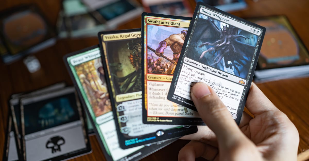
Exploring Shuffle Count and Randomness: How Many Times Should a Magic: The Gathering Player Shuffle?
Note: This article was translated from Chinese by AI and may contain errors. Read the original Chinese version.
1. Introduction: Why Study “How Many Shuffles Are Enough”?
In card games, whether with playing cards or Magic: The Gathering (hereafter MTG), shuffling is a common action. But how many shuffles does it actually take to ensure the card order is mixed to near randomness? And this is critical to game balance.
- Playing cards usually come as 52 cards, and general research finds that 7 to 8 shuffles is quite random.
- An MTG deck usually has 60 cards (excluding the sideboard). In this case, the number of shuffles may also need slight adjustment, to ensure that the “opening hand,” “draw order” and so on are not affected by any predictable pattern.
Especially for MTG players, it’s not just about plain “fairness”; you also want to avoid extreme situations such as “land clumps or droughts” caused by improper shuffling (colloquially called mana screw or mana flood). This article gives a simple look at how, with a 60-card MTG deck, we should think about the number of shuffles needed to shuffle randomly enough, and explores how to measure randomness mathematically.
2. Brief Conclusion and Practical Advice
- Advice for MTG players: To avoid an unfair opening hand or having your land and mana distribution guessed, we recommend at least 6 shuffles. If you shuffle casually, it’s safest to do 9 or more.
3. Why Should MTG Players Care About Shuffle Randomness?
Many MTG players may have thought: “Three or five shuffles is enough, right?” But when a deck’s structure cares about the curve and mana configuration, and the card order must be unpredictable during tournament matches, you must ensure the shuffle is truly random. There are several reasons here:
- Ensuring fairness of the “opening seven”
You don’t want certain key cards to be overly concentrated because cards may be “partly stacked together.” - Referring to the playing-card literature
Bayer & Diaconis (1992), studying 52 cards, mention that “7 riffle shuffles” is almost enough. So for MTG’s 60 cards, would 7 to 9 shuffles do?
If the shuffle isn’t random enough, someone with bad intentions might “track cards” or “manipulate the deck”; too many shuffles waste precious tournament or casual time, so the “optimal number of shuffles” is an important research topic.
4. Background Theory: How Do We Measure “Randomness”?
To judge whether something is “random enough,” we first need a quantitative measure. Two approaches are common in research:
- Variation Distance
Let Q(pi) denote the probability of each card order pi appearing after shuffling, and U(pi) the ideal probability under perfect uniformity (that is, 1 / (n!)). Then define:
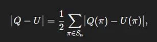
Here n = 60 (for MTG), and S_n denotes all possible permutations (n! in total). If this distance is small enough, we can say it is “almost the same as ideal randomness.” Unfortunately, the mathematics of variation distance is rather difficult and writing a program for it is troublesome, so we can use another method instead.
- Chi-square Test
Simulate a large number of shuffle results and compare them with the “perfectly random” distribution, using the chi-square statistic:
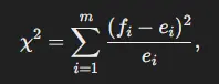
to observe whether it is close to the ideal distribution. f_i is the observed count falling in category i in the experiment, and e_i is the theoretical expected count. If X^2 is smaller than the critical value, the shuffled card order is “random enough.”
The core of this article focuses on the chi-square test approach, which makes it convenient for us to find the key shuffle count from a simulation perspective.
5. Core Idea: Number of Shuffles vs. Randomness
Whether 52 or 60 cards, the key is “how many shuffles” it takes to approach the ideal distribution.
- 1 to 2 shuffles: usually leave obvious bias, and a perceptive opponent can catch traces of an incomplete shuffle.
- About 7 to 8 shuffles: for a 52-card playing deck, theoretical models show this is almost random enough. For a 60-card MTG deck, a few more shuffles may be needed.
- 10 to 11 shuffles or more: further shuffling brings limited gains, because after this point the “randomness” curve is already saturated.
6. Research Results and Conclusion
In shuffling research on 52 playing cards, the conclusion proposed by Bayer and Diaconis states that after 7 consecutive random shuffles, the arrangement of the playing cards reaches a level of “no significant difference from perfectly random.” This also echoes the earlier inference of Bayer & Diaconis (1992): the number of shuffles is approximately (3/2(logN/log2). Plugging in (n = 52), the computed value is roughly 8.8, not far from the actual experimental result (7 being sufficient).
This study uses the same theoretical basis, changing the playing cards to a 60-card MTG deck (most basic deck designs are about 60 cards), and runs large-scale computer simulations and chi-square tests to explore the number of shuffles needed to go “from the initial state to nearly perfectly random.” In theory, the formula of Aldous and Bayer & Diaconis gives 9 (3/2(logN/log2), N=60), meaning about 9 shuffles should reach near-maximal randomness. However, the actual simulation results show that about 6 to 7 random shuffles already make “the rearrangement of the whole 60-card deck” and “the ideal perfectly random arrangement” show no significant difference.
1. Simulation and Testing Methods
Program simulation
- To accurately estimate the effect of the shuffle count, this study ran a total of 200,000 simulations of the “random cut-point shuffle (riffle shuffle).”
- Each run starts from a “fixed initial arrangement”; after (k) consecutive shuffles, the “distance” (total_distance) between the final card order and the initial arrangement is recorded.
- Shuffle method model:
Cut
- The cut position is set “roughly” at the exact middle. Then the amount by which the cut position “deviates” from the center is set, using a standard deviation of 0.3 (30% overall). Finally, it ensures each half has at least a few cards (default minimum of 5 in the program)
Riffle
- Decide the probability distribution of “how many cards to drop from the left” or “from the right” at a time.
- 60% chance of dropping only 1 card
- 25% chance of dropping 2 cards at once
- 15% chance of dropping 3 cards at once
- The program first takes 1 to 3 cards from the left pile into the new pile, then 1 to 3 cards from the right pile into the new pile, alternating like this until both piles are used up.
- Decide the probability distribution of “how many cards to drop from the left” or “from the right” at a time.
- Repeat the above procedure, and stably estimate the card order distribution for each shuffle count through large-scale sampling (tens of thousands).
- Using the total_distance after each shuffle as the indicator, group the values and perform a chi-square test against the distance distribution under perfect randomness.
- Null hypothesis (H0): The distribution for that shuffle count has no significant difference from the perfectly random distribution.
- Significance level (α): 0.05.
- If the test result is p-value > 0.05, that is “fail to reject H0,” meaning that shuffle count is enough to bring the card order to a level with no significant difference from perfectly random.
Note 1, the concept of the riffle shuffle:
- Splitting: Imagine you have a deck in your hands and split it into two piles. This action is like using your thumb and other fingers to separate the deck into two parts.
- Interleaving: Next, randomly drop one to three cards alternately from these two piles, recombining them into one deck. This process is like aligning the edges of the two piles and then gently letting the cards fall interleaved with your fingers.
>

2. Simulation Analysis Results
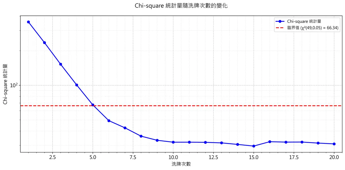
The table below consolidates the chi-square test statistic (Chi2_stat), degrees of freedom (DOF) and p-value for 0 to 20 shuffles, as well as the descriptive statistics of the simulated distribution (Mean, Std, Q1, Median, Q3, Min, Max).
Note 2: Here the degrees of freedom (DOF) of the X^2 test defaults to 49, and does not apply to the perfectly random case.
| Shuffles | X^2_stat | p_value | Reject H0 |
|---|---|---|---|
| 1 | 355.9 | 0.00 | Yes |
| 2 | 234.9 | 0.00 | Yes |
| 3 | 152.5 | 0.00 | Yes |
| 4 | 100.6 | 0.00 | Yes |
| 5 | 67.5 | 0.04 | Yes |
| 6 | 49.2 | 0.47 | No |
| 7 | 42.6 | 0.73 | No |
| 8 | 36.0 | 0.92 | No |
| 9 | 33.2 | 0.96 | No |
| 10 | 31.9 | 0.97 | No |
| 11 | 32.0 | 0.97 | No |
| 12 | 31.9 | 0.97 | No |
| — | — | — | — |
| 20 | 30.9 | 0.98 | No |
From the table we can see:
- For 1 to 5 shuffles, the p-value is all below 0.05, meaning there is a “significant difference from perfectly random” at that point.
- Starting from 6 shuffles, the p-value rises to 0.4663, above 0.05, meaning “no significant difference from perfectly random.”
- As the shuffle count increases further, the p-value mostly stays above 0.05, showing the arrangement distribution has become close to the “ideal perfect randomness.”
3. Final Recommendations
Simulation results:
- This experiment shows that for a 60-card MTG deck, shuffling consecutively 6 or more times from the initial arrangement reaches the level of “not rejecting that it is the same as the perfectly random distribution” in the chi-square test.
Recommendations and limitations:
- For ordinary games with friends or more casual events, 5 to 6 shuffles give decent randomness.
- For official tournaments or when you want to eliminate the effects of “memory, prediction” and the like as much as possible, consider following the theoretically recommended 8 to 9 shuffles or even more.
- The above conclusions still depend on the assumption of the “random cut-point shuffle (riffle shuffle).” According to research, cutting, the Hindu shuffle and wash shuffles can hardly achieve randomness, which may result in insufficient actual randomness.
7. References

- Title
- Exploring Shuffle Count and Randomness: How Many Times Should a Magic: The Gathering Player Shuffle?
- Author
- mm
- Created at
- February 10, 2025
- License
- This work is licensed under CC BY-NC-SA 4.0 .